25 May 2021
First, a typical set up. You can dowload the data from here, as well as the code itself.
* WorkingDirectory
cd "your-directory"
* Packages
*net install grc1leg, from(http://www.stata.com/users/vwiggins) /* many graphs, one legend */
* Load data
clear all
use russiaAmong different variables we’ve got these:
.   describe satlif marsta* gender

              storage   display    value
variable name   type    format     label      variable label
─────────────────────────────────────────────────────────────────────────────
satlif          double  %10.0g                Satisfaction with Life
marsta1         float   %9.0g                 Married
marsta2         float   %9.0g                 Living Together
marsta3         float   %9.0g                 Divorced
marsta4         float   %9.0g                 Widowed
gender          double  %10.0g                Male
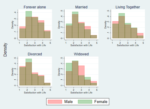
I’m curious about satisfaction with life. Does marital status have relation with it? Does gender? Let’s do some plots
egen temp = rowtotal(marsta*)
gen marsta0 = 1-temp
label variable marsta0 "Forever alone"
drop temp
Now a cool loop
forvalues k = 0(1)4{
  local titulo : variable label marsta`k'
  twoway (histogram satlif if gender==1 & marsta`k'==1, bin(5) color(red%30)) ///
       (histogram satlif if gender==0 & marsta`k'==1, bin(5) color(green%30)), ///
        name(H_`k') title("`titulo'") legend(order(1 "Male" 2 "Female" ))
}
quietly graph dir H_*
grc1leg `r(list)', l1(Density) legendfrom(H_1)
graph close H_*It looks interesting…
Another interesting looking thing, is the variable:
. describe hhpres

              storage   display    value
variable name   type    format     label      variable label
─────────────────────────────────────────────────────────────────────────────
hhpres          double  %10.0g                Others Present at Interview
Does people that ansewred the questions with someone else close to have different answers to those who were alone? In which variables? Let’s see:
ds hhpres, not
foreach v of varlist `r(varlist)' {
    quietly ttest `v', by(hhpres)
    if r(p)<0.01 {
        display "`: var label `v''"
    }
}
Site Male Age (in months) Health Prob last 30 days Self-reported Height Ever Had Heart Attack Smokes Height HH Income Real Geographic Area Married Divorced Widowed
Suppose that we want to explain a continuous variable using another continuous variable, so we don’t have many options:
. describe totexp monage htself tincm_r

              storage   display    value
variable name   type    format     label      variable label
─────────────────────────────────────────────────────────────────────────────
totexpr         double  %10.0g                HH Expenditures Real
monage          double  %10.0g                Age (in months)
htself          double  %10.0g                Self-reported Height
tincm_r         double  %10.0g                HH Income Real
reg totexp monage Source │ SS df MS Number of obs = 2,44
─────────────┼────────────────────────────────── F(1, 2445) = 86.4
Model │ 6.5927e+09 1 6.5927e+09 Prob > F = 0.000
Residual │ 1.8652e+11 2,445 76284541.1 R-squared = 0.034
─────────────┼────────────────────────────────── Adj R-squared = 0.033
Total │ 1.9311e+11 2,446 78948635.7 Root MSE = 8734.
─────────────┬───────────────────────────────────────────────────────────────
totexpr │ Coef. Std. Err. t P>|t| [95% Conf. Interval
─────────────┼───────────────────────────────────────────────────────────────
monage │ -7.666014 .824627 -9.30 0.000 -9.283053 -6.04897
_cons │ 11921.72 491.9559 24.23 0.000 10957.03 12886.4
─────────────┴───────────────────────────────────────────────────────────────
Let’s do bad things and over-fit the regression using a polynomial. In fact, let’s see how R^2 changes while the degree of the polynomial rises.
quietly matrix mat_r = J(10,2,.)
quietly forvalues k = 1(1)10{
    quietly gen monage_`k' = monage^`k'
    quietly ds monage_*
    quietly reg totexp `r(varlist)'
    quietly matrix mat_r[`k',2] = e(r2)
    quietly matrix mat_r[`k',1] = `k'
}
drop _all
svmat double mat_r
matrix drop mat_r
twoway connected mat_r2 mat_r1, ytitle("R{sup:2}") xtitle("Polynomial degree")
use russia, clear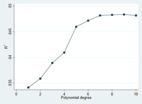
To be continued…