Soy price

A non-rigorous example

We begin by importing the data we are goin to use. You can dowload the data from here.

clear all
import delimited "folder-containing-the-file\psoy.csv"

We must add a month variable, and give time series format

gen month=monthly(mes,"YM")
format month %tm
tsset month

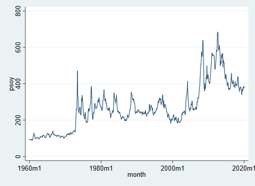
Let’s plot our data

tsline psoy

The above time series si not stationary at all. So we apply logaritmic difference:

gen lns=ln(psoy)
gen dlns=D.lns
tsline dlns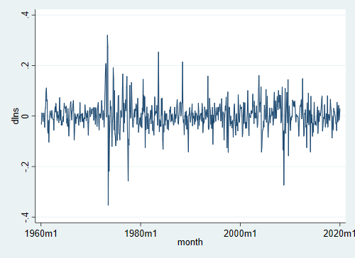

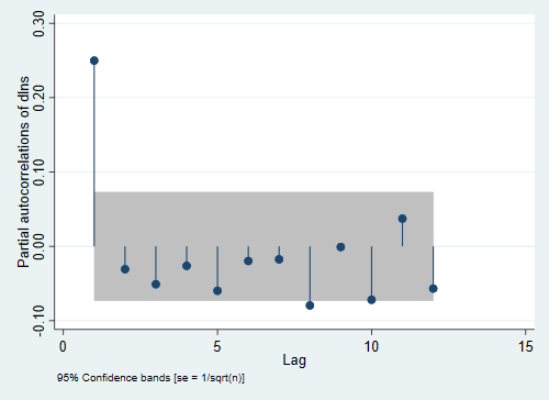
Is it auto correlated?

corrgram dlns, lags(12)
ac dlns, lags(12)
pac dlns, lags(12)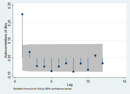

Let’s try to estimate an AR(1)

arima dlns, ar(1)

(setting optimization to BHHH)
Iteration 0:   log likelihood =   1067.751  
Iteration 1:   log likelihood =  1067.7511  
Iteration 2:   log likelihood =  1067.7511  
Iteration 3:   log likelihood =  1067.7511  
Iteration 4:   log likelihood =  1067.7511  

ARIMA regression

Sample:  1960m2 - 2020m1                        Number of obs     =        720
                                                Wald chi2(1)      =     149.70
Log likelihood =  1067.751                      Prob > chi2       =     0.0000

─────────────┬────────────────────────────────────────────────────────────────
             │                 OPG
        dlns │      Coef.   Std. Err.      z    P>|z|     [95% Conf. Interval]
─────────────┼────────────────────────────────────────────────────────────────
dlns         │
       _cons │   .0019588   .0028895     0.68   0.498    -.0037045     .007622
─────────────┼────────────────────────────────────────────────────────────────
ARMA         │
          ar │
         L1. │   .2495429   .0203956    12.24   0.000     .2095683    .2895176
─────────────┼────────────────────────────────────────────────────────────────
      /sigma │   .0549165   .0006728    81.62   0.000     .0535979    .0562352
─────────────┴────────────────────────────────────────────────────────────────
Note: The test of the variance against zero is one sided, and the two-sided
      confidence interval is truncated at zero.

Are its residuals white noise?

predict resid_ar1, resid
wntestq resid_ar1

Portmanteau test for white noise
───────────────────────────────────────
 Portmanteau (Q) statistic =    55.4994
 Prob > chi2(40)           =     0.0524

Let’s se visually how acurate are the fitted values

predict dlns_ar1
tsline dlns dlns_ar1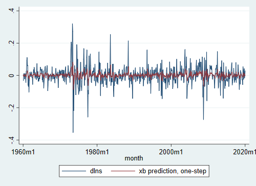

This code is just an example, in order to developed a better model one should follow the Box-Jenknis method.